Agency Prepayment Commentary Report
(415)710-8689
help@cprcdr.com
Using: June 2026 Agency flash reports parsed as text-formatted .xls files
1. Data ingest and template binding
The four June 2026 Agency flash files were treated as plain-text tables rather than Excel workbooks. The commentary structure follows the attached Agency Prepayment Commentary Report format: data ingest, aggregate coupon stack, main prepayment signal, product interpretation, dealer matrix, governance status, and final dealer line.
Files parsed: fn_flash_rpt_202606.xls; fh_flash_rpt_202606.xls; g1_flash_rpt_202606.xls; g2_flash_rpt_202606.xls.
Parsed fields: Product | Coupon | OYear | CBal($MM) | WAC | WAM | WALA | Cpr1 | Cpr1Prev | 1Mo%Chg | Cpr3 | Cpr6 | Cpr12.
Total parsed rows: 1,155; total reported balance: $11,466,059MM.
2. Aggregate coupon stack — weighted CPR
| Coupon | Balance $MM | Weighted CPR1 | CPR1 Prev | Mo Delta | CPR3 | CPR6 | CPR12 | Desk Signal |
|---|
| 1.0 | 5,270 | 4.70 | n/a | n/a | 4.21 | 3.81 | 3.88 | HOLD ONLY / HEDGE |
| 1.5 | 334,242 | 4.77 | 7.91 | -3.14 | 4.51 | 3.95 | 4.11 | HOLD ONLY / HEDGE |
| 2.0 | 2,233,251 | 5.50 | 5.26 | +0.23 | 5.16 | 4.56 | 4.78 | HOLD ONLY / HEDGE |
| 2.5 | 1,845,789 | 6.61 | 6.46 | +0.15 | 6.29 | 5.68 | 5.89 | HOLD ONLY / HEDGE |
| 3.0 | 1,349,436 | 6.95 | 6.72 | +0.23 | 6.68 | 6.14 | 6.36 | HOLD ONLY / HEDGE |
| 3.5 | 1,067,559 | 7.09 | 7.07 | +0.02 | 6.94 | 6.40 | 6.63 | HOLD / ADD ON WIDENING |
| 4.0 | 804,741 | 7.52 | 7.58 | -0.05 | 7.39 | 6.83 | 6.94 | HOLD / ADD ON WIDENING |
| 4.5 | 666,082 | 7.53 | 7.66 | -0.12 | 7.55 | 6.74 | 6.63 | ADD / DEFENSIVE BUY |
| 5.0 | 982,762 | 7.90 | 8.24 | -0.34 | 8.44 | 7.54 | 6.64 | BUY / CORE LONG |
| 5.5 | 1,035,629 | 12.00 | 14.73 | -2.74 | 15.55 | 14.41 | 12.88 | TRIM / SELECTIVE ONLY |
| 6.0 | 752,829 | 19.16 | 23.83 | -4.67 | 24.86 | 24.02 | 21.44 | SELL / AVOID GENERIC |
| 6.5 | 304,988 | 25.83 | 31.09 | -5.26 | 31.20 | 30.26 | 27.75 | SELL / AVOID GENERIC |
| 7.0 | 73,432 | 30.55 | 34.54 | -3.98 | 35.18 | 34.82 | 33.09 | SELL / AVOID GENERIC |
| 7.5 | 9,752 | 28.39 | 32.35 | -3.96 | 30.55 | 28.94 | 28.48 | SELL / AVOID GENERIC |
| 8.0 | 297 | 28.94 | 20.97 | +7.97 | 23.91 | 23.41 | 26.83 | SELL / AVOID GENERIC |
June tape read-through: the broad coupon stack remains turnover-driven rather than refinance-driven. The main change versus the prior commentary template is cleaner premium deceleration: 5.5, 6.0, 6.5, and 7.0 all slowed month-over-month, but absolute premium speeds are still too high for generic buying.
3. Main prepayment signal
A. Current coupon remains the cleanest long
The 5.0 coupon is still the preferred dealer bucket: CPR1 = 7.90, down from 8.24, with month delta = -0.34 and CPR12 = 6.64. That means the 5.0 stack still has useful income, controlled speeds, moderated convexity risk, and better premium-retention than the 5.5+ stack.
Desk read: 5.0 specified pools remain the core long; avoid replacing this with a broad generic MBS beta trade.
B. 4.5 is the defensive add zone
The 4.5 coupon ran CPR1 = 7.53, slightly below prior-month CPR1 of 7.66. CPR12 is 6.63, which keeps the bucket in a defensive-carry profile rather than a high-premium burn profile.
Desk read: 4.5 = add selectively / defensive buy, especially when OAS cushion is visible.
C. 5.5+ remains premium-risk even after deceleration
Premium speeds slowed materially: 5.5 CPR1 = 12.00, 6.0 CPR1 = 19.16, 6.5 CPR1 = 25.83, and 7.0 CPR1 = 30.55. However, the absolute speeds are still high enough to create premium-burn and convexity risk.
Desk read: trim 5.5 unless specified collateral is exceptional; sell/avoid 6.0+ generic premium collateral.
D. Low coupons remain extension assets
Low coupons remain slow: 2.0 CPR1 = 5.50, 2.5 CPR1 = 6.61, and 3.0 CPR1 = 6.95. They carry low refinance risk but also embed high duration and extension risk.
Desk read: hold only as extension-hedged ballast; do not add aggressively without spread compensation or a clean duration hedge.
4. Agency / product interpretation
Conventional FN/FH
Conventional FN/FH remains the cleaner long expression than GNMA II premium exposure. Conventional 30-year 5.0 speeds are still near the controlled current-coupon zone, while conventional 5.5+ speeds slow but remain premium-risky. Freddie 30-year high coupons look optically slower in some buckets, but balances are much smaller, so liquidity and cohort selection matter.
Desk read: FN/FH specified 5.0 remains preferred; use 4.5 as defensive carry; avoid broad high-premium beta.
GNMA I
G130 5.0: balance $4,558MM, CPR1 7.40, CPR12 7.15.
G130 5.5: balance $2,456MM, CPR1 7.15, CPR12 6.45.
G130 6.0: balance $2,078MM, CPR1 8.39, CPR12 6.99.
GNMA I high coupons are still optically slower than GNMA II, but the balances are smaller and the trade should be treated as niche / liquidity-sensitive rather than a generic premium overweight.
GNMA II
G230 5.0: balance $322,735MM, CPR1 7.25, CPR12 6.57.
G230 5.5: balance $359,502MM, CPR1 14.64, CPR12 15.39.
G230 6.0: balance $239,186MM, CPR1 25.81, CPR12 25.68.
G230 6.5: balance $103,160MM, CPR1 30.47, CPR12 28.98.
G230 7.0: balance $27,298MM, CPR1 33.17, CPR12 33.05.
GNMA II remains the fastest premium stack. G230 5.5+ should remain an avoid / RV-short bucket against UMBS 5.0 unless live OAS is unusually compelling.
5. Dealer Buy / Sell matrix by coupon
| Coupon | Dealer Signal | Rationale |
|---|
| 1.5 | HOLD ONLY / HEDGE | Extension-heavy; low refi risk but duration/extension risk dominates. |
| 2.0 | HOLD ONLY / HEDGE | Extension-heavy; low refi risk but duration/extension risk dominates. |
| 2.5 | HOLD ONLY / HEDGE | Extension-heavy; low refi risk but duration/extension risk dominates. |
| 3.0 | HOLD ONLY / HEDGE | Extension-heavy; low refi risk but duration/extension risk dominates. |
| 3.5 | HOLD / ADD ON WIDENING | Transition zone; modest speeds but still duration-sensitive. |
| 4.0 | HOLD / ADD ON WIDENING | Defensive carry; clean but not as income-rich as 4.5/5.0. |
| 4.5 | ADD / DEFENSIVE BUY | Best defensive current-coupon sleeve; speeds stable and not premium-burn heavy. |
| 5.0 | BUY / CORE LONG | Cleanest carry bucket; CPR eased and income is still useful. |
| 5.5 | TRIM / SELECTIVE ONLY | Premium risk still elevated despite meaningful speed deceleration. |
| 6.0 | SELL / AVOID GENERIC | High absolute CPR and convexity/premium-burn risk remain severe. |
| 6.5 | SELL / AVOID GENERIC | High absolute CPR and convexity/premium-burn risk remain severe. |
| 7.0 | SELL / AVOID GENERIC | High absolute CPR and convexity/premium-burn risk remain severe. |
6. Updated Agency commentary
The June 2026 flash tape confirms that the Agency market remains in a turnover-driven, not refinance-driven, prepayment regime. Current-coupon collateral continues to offer the cleanest carry profile, while high-premium coupons remain exposed to convexity and premium-burn risk. The key change is that premium speeds are decelerating, but the absolute CPR level in 5.5+ is still too fast to justify broad generic premium buying.
Dealer conclusion: Buy 5.0 specified pools. Add 4.5 selectively. Hold low coupons only as extension-hedged ballast. Trim 5.5. Sell / avoid 6.0–7.0 generic premium collateral.
7. Gravitas / Agency Alpha Pack mapping
The uploaded Gravitas dictionary contains the Agency Alpha lane: AGENCY_ALPHA_ENGINE_GRAMMAR_V1, AGENCY_ALPHA_STATE_INGEST_V1, AGENCY_CPR_FORECAST_BLEND_V1, AGENCY_OAS_MONTE_CARLO_PROXY_V1, AGENCY_RV_ZSCORE_SURFACE_BUILD_V1, AGENCY_TBA_ROLL_CARRY_DECOMPOSE_V1, AGENCY_ALPHA_HEDGE_OPTIMIZER_V1, AGENCY_ALPHA_SIGNAL_FUSE_V1, AGENCY_ALPHA_STATUS_COLLAPSE_V1, and AGENCY_ALPHA_EMIT_EVIDENCE_PACK16_V1. For this report, those operators are used as a commentary governance frame rather than as live-trading authorization.
vplus237 layer Agency report binding
Pack_O Flash CPR tables, coupon balances, WAC/WAM/WALA, product family, monthly speed change.
Pack_M_step CPR blend, premium-burn read, extension-risk read, coupon stack RV proxy, carry/roll interpretation.
Pack_U Candidate routes: BUY 5.0, ADD 4.5, HOLD/HEDGE low coupons, TRIM 5.5, SELL/AVOID 6.0+.
Pack_G Audit trace: source files, parsed row count, text-file ingest, no live OAS/hedge book, telemetry-only status.
8. 404 verifier
| Gate | Status | Reason |
|---|
| Flash CPR ingest | GREEN | Four text-formatted flash reports parsed successfully. |
| CPR consistency | GREEN | Coupon stack behavior is coherent; current coupon controlled, premium decelerating but still fast. |
| Product-family coherence | GREEN | Conventional 5.0 is cleaner; GNMA II premiums remain fastest. |
| OAS validation | YELLOW | Dealer live OAS marks are not attached. |
| Hedge bounds | YELLOW | No live risk book, DV01, convexity, or hedge sleeve attached. |
| RV consistency | YELLOW | RV proxy inferred from CPR and balances; live TBA/spec-pool marks not attached. |
| Execution authorization | RED | No live release authority; commentary only. |
Final status
ACTION_MODE = TELEMETRY_ONLY
LIVE_ROUTING = BLOCKED
PACK_U_COMMIT = DENY UNTIL 404 GREEN
Final Dealer Line
Agency MBS desk should be long selective current coupon, not long generic MBS beta.
Best expression:
BUY 5.0 specified pools
ADD 4.5 defensively
HOLD low coupons with extension hedge
TRIM 5.5 unless collateral is strongly specified and OAS is compelling
SELL / AVOID 6.0–7.0 generic premium collateral
This is still not a pure "rates down = buy MBS" trade. The right output remains: buy selectively, demand OAS cushion, hedge convexity, and treat liquidity/QT drag as the hidden spread risk. Current-coupon Agency MBS can generate carry alpha, but only when spreads compensate for convexity risk and only with explicit hedge discipline and governance controls.
Appendix A. Product-family premium coupon detail
| Product | Coupon | Balance $MM | CPR1 | Prev | CPR12 |
|---|
| Conv 5/1 Hybrid | 6.0 | 1,890 | 12.99 | 16.00 | 14.15 |
| Conv 7/1 Hybrid | 6.0 | 2,395 | 14.71 | 15.38 | 16.26 |
| Conv15 | 4.0 | 10,099 | 10.15 | 10.58 | 8.69 |
| Conv15 | 4.5 | 12,377 | 11.27 | 11.87 | 10.53 |
| Conv15 | 5.0 | 13,899 | 16.77 | 17.12 | 17.92 |
| Conv15 | 5.5 | 9,479 | 19.11 | 21.45 | 19.51 |
| Conv15 | 6.0 | 4,583 | 24.34 | 25.28 | 23.45 |
| Conv30 | 4.0 | 389,120 | 7.51 | 7.54 | 6.99 |
| Conv30 | 4.5 | 262,324 | 7.59 | 7.83 | 6.94 |
| Conv30 | 5.0 | 352,821 | 7.90 | 8.08 | 6.28 |
| Conv30 | 5.5 | 370,568 | 10.36 | 13.29 | 11.30 |
| Conv30 | 6.0 | 278,558 | 15.96 | 21.52 | 19.41 |
| Conv30 | 6.5 | 114,664 | 23.54 | 30.16 | 27.22 |
| Conv30 | 7.0 | 27,111 | 29.02 | 34.08 | 33.19 |
| FH30 | 4.0 | 60,766 | 7.13 | 7.54 | 7.10 |
| FH30 | 4.5 | 27,832 | 7.85 | 8.54 | 7.94 |
| FH30 | 5.0 | 10,046 | 8.00 | 8.73 | 8.28 |
| FH30 | 5.5 | 4,761 | 8.20 | 9.18 | 8.07 |
| FH30 | 6.0 | 3,058 | 7.84 | 9.69 | 7.96 |
| FN 5/1 Hybrid | 6.0 | 1,490 | 13.97 | 16.71 | 14.58 |
| FN 7/1 Hybrid | 6.0 | 1,901 | 15.19 | 14.56 | 16.43 |
| FN 10/1 Hybrid | 4.0 | 1,439 | 6.80 | n/a | 5.80 |
| FN 10/1 Hybrid | 4.5 | 4,194 | 8.24 | n/a | 5.31 |
| FN 10/1 Hybrid | 5.0 | 6,414 | 8.57 | n/a | 10.09 |
| FN 10/1 Hybrid | 5.5 | 2,398 | 13.12 | 0.85 | 18.98 |
| FN 10/1 Hybrid | 6.0 | 2,650 | 15.18 | 21.60 | 17.40 |
| FN15 | 4.0 | 6,708 | 9.35 | 9.37 | 7.55 |
| FN15 | 4.5 | 10,740 | 11.07 | 11.49 | 10.36 |
| FN15 | 5.0 | 10,999 | 17.15 | 15.90 | 18.30 |
| FN15 | 5.5 | 6,756 | 19.76 | 19.33 | 19.19 |
| FN15 | 6.0 | 2,986 | 24.70 | 23.86 | 22.54 |
| FN30 | 4.0 | 179,648 | 7.55 | 7.45 | 6.78 |
| FN30 | 4.5 | 150,753 | 7.41 | 7.61 | 6.47 |
| FN30 | 5.0 | 255,907 | 7.71 | 7.67 | 5.87 |
| FN30 | 5.5 | 277,375 | 10.35 | 12.74 | 11.38 |
| FN30 | 6.0 | 210,882 | 16.16 | 21.03 | 19.88 |
| FN30 | 6.5 | 82,949 | 23.69 | 30.49 | 27.49 |
| FN30 | 7.0 | 18,797 | 29.11 | 34.59 | 33.30 |
| G130 | 4.0 | 6,754 | 6.63 | 6.98 | 6.07 |
| G130 | 4.5 | 6,745 | 7.42 | 7.37 | 6.65 |
| G130 | 5.0 | 4,558 | 7.40 | 7.09 | 7.15 |
| G130 | 5.5 | 2,456 | 7.15 | 7.31 | 6.45 |
| G130 | 6.0 | 2,078 | 8.39 | 8.97 | 6.99 |
| G2 5/1 Hybrid | 4.0 | 2,449 | 1.72 | 1.82 | 0.79 |
| G2 5/1 Hybrid | 4.5 | 4,965 | 3.93 | 4.48 | 1.42 |
| G2 5/1 Hybrid | 5.0 | 3,502 | 12.15 | 14.01 | 7.04 |
| G2 5/1 Hybrid | 5.5 | 1,000 | 20.35 | 23.27 | 15.40 |
| G215 | 4.5 | 1,416 | 11.27 | 11.10 | 7.31 |
| G215 | 5.0 | 1,545 | 17.74 | 17.92 | 14.56 |
| G230 | 4.0 | 145,627 | 7.54 | 7.59 | 6.94 |
| G230 | 4.5 | 184,519 | 7.09 | 6.87 | 5.81 |
| G230 | 5.0 | 322,735 | 7.25 | 8.11 | 6.57 |
| G230 | 5.5 | 359,502 | 14.64 | 17.58 | 15.39 |
| G230 | 6.0 | 239,186 | 25.81 | 29.56 | 25.68 |
| G230 | 6.5 | 103,160 | 30.47 | 33.10 | 28.98 |
| G230 | 7.0 | 27,298 | 33.17 | 35.13 | 33.05 |
9. Fat-tail risk overlay
The base report correctly identifies June 2026 as a turnover-driven, not refinance-driven, prepayment tape. The fat-tail overlay adds a stress discipline: the desk should not underwrite only the observed one-month deceleration in premium speeds. Premium coupons still sit on a convex payoff surface where a rates rally, servicer buyout wave, borrower credit normalization, or liquidity shock can create nonlinear premium-burn. Low coupons carry the opposite tail: duration extension and hedge slippage if rates back up or volatility rises. The correct risk posture is therefore barbell-aware rather than beta-long: own controlled current coupon; hedge extension in low coupons; avoid generic premium convexity tails.
| Tail scenario | Primary exposure | Impact path | Risk-control implication |
|---|
| Fast refi / rally tail | 5.5–7.0 premium coupons | CPR can jump from already-high levels; premium amortization accelerates and convexity turns adverse. | Sell/avoid 6.0+ generic; trim 5.5 unless specified collateral and OAS cushion are strong. |
| Servicer / buyout tail | GNMA II premium stack | Buyout behavior can make GNMA II premium speeds remain faster than UMBS even when headline speeds decelerate. | Keep G230 5.5+ as RV-short/avoid bucket against UMBS 5.0. |
| Extension tail | 1.5–3.0 low coupons | Slow CPR plus rate backup increases duration, hedge cost, and negative carry risk. | Hold only as extension-hedged ballast; do not add without spread compensation. |
| Liquidity / QT tail | Generic MBS beta and small-balance niches | Spread widening can overwhelm carry; smaller GNMA I/FH high-coupon cohorts may not exit cleanly. | Prefer liquid FN/FH specified 5.0; demand liquidity premium for niche pools. |
| Model misspecification tail | All coupons | Month-over-month CPR deceleration may be temporary; point-estimate CPR can understate path dispersion. | Use scenario bands and 404 governance; do not treat telemetry as live-trading authorization. |
10. Relative value analysis
RV is framed as carry-after-tail-risk, not raw coupon yield. The best long is the bucket with enough income, controlled CPR, manageable convexity, and liquid execution. On this tape, 5.0 specified pools remain the cleanest RV long because CPR1 eased to 7.90 and CPR12 is 6.64, while income is still useful. The 4.5 coupon is the defensive add because speeds are stable and premium-burn is limited. The 5.5 coupon is no longer an outright short in every specified cohort, but it is still a trim/selective-only bucket because absolute CPR remains 12.00 and three-month CPR is 15.55. The 6.0–7.0 stack is still poor RV generically: even after deceleration, CPR1 remains 19.16 to 30.55 and CPR12 remains 21.44 to 33.09.
| Bucket | RV grade | Fat-tail grade | Recommended expression | Reason |
|---|
| 4.5 | Positive / defensive | Low-moderate | Add selectively | Stable CPR and defensive carry; add only when OAS cushion is visible. |
| 5.0 | Best positive RV | Moderate | Core long in specified pools | Best balance of income, controlled CPR, liquidity, and lower premium-burn than 5.5+. |
| 5.5 | Mixed / cohort-specific | High | Trim; selective specified only | Deceleration is real, but absolute CPR and CPR3 are still too fast for generic overweight. |
| 6.0 | Negative generic RV | Very high | Sell / avoid generic | Premium burn and convexity dominate; GNMA II 6.0 is especially exposed. |
| 6.5–7.0 | Strong negative generic RV | Extreme | Sell / avoid generic | Fast absolute CPR and adverse convexity leave poor carry-after-tail-risk. |
| 1.5–3.0 | Neutral only if hedged | Extension high | Hold as hedged ballast | Slow speeds reduce refi risk but duration extension dominates. |
11. Product RV and pair-trade read
| RV trade | Long leg | Short / underweight leg | Why this is cleaner |
|---|
| Current-coupon carry RV | FN/FH specified 5.0 | Generic 6.0+ premium collateral | Captures controlled carry while reducing exposure to fast premium CPR tails. |
| Defensive carry sleeve | 4.5 specified collateral | 5.5 generic premium beta | Uses stable 4.5 speeds against 5.5 premium-burn uncertainty. |
| GNMA premium RV | UMBS 5.0 or high-quality specified FN/FH | G230 5.5–6.5 generic | GNMA II remains the fastest premium stack; RV-short remains justified unless OAS is exceptional. |
| Low-coupon hedge sleeve | 1.5–3.0 only with duration hedge | Unhedged low-coupon duration | Avoids extension tail being mistaken for cheap carry. |
12. Updated risk-adjusted dealer matrix
| Coupon | Base signal | Fat-tail adjustment | RV-adjusted dealer line |
|---|
| 1.5–3.0 | Hold only / hedge | Extension tail remains the dominant risk. | Hold only with explicit duration hedge; add only on major widening. |
| 3.5–4.0 | Hold / add on widening | Moderate extension risk; limited premium burn. | Accumulate only when spread/OAS compensates hedge cost. |
| 4.5 | Add / defensive buy | Best defensive sleeve; still subject to liquidity spread tail. | Add selectively; prefer specified collateral with OAS cushion. |
| 5.0 | Buy / core long | Cleanest carry-after-tail-risk, but avoid generic beta sizing. | Core long in specified pools; pair against 6.0+ premium shorts/underweights. |
| 5.5 | Trim / selective only | Absolute CPR remains elevated despite deceleration. | Trim generic; own only strong specified cohorts with compelling OAS. |
| 6.0–7.0 | Sell / avoid generic | Extreme premium-burn and convexity tail. | Sell/avoid generic; use as RV short versus UMBS 5.0. |
13. Revised 404 verifier after fat-tail and RV overlay
| Gate | Status | Reason |
|---|
| Fat-tail scenario coverage | GREEN | Rally/refi, servicer buyout, extension, liquidity/QT, and model-miss tails are explicitly identified. |
| RV ranking | GREEN | 5.0 specified remains best positive RV; 4.5 defensive add; 6.0+ generic remains negative RV. |
| Product-pair coherence | GREEN | UMBS/FN/FH specified 5.0 versus G230 5.5+ premium underweight is internally consistent with speed data. |
| Live OAS validation | YELLOW | No live dealer marks, pool payups, TBA roll levels, or hedge book are attached. |
| Execution authorization | RED | This remains telemetry-only commentary, not live-trading authorization. |
Final risk-adjusted dealer line
After applying fat-tail and RV analysis, the conclusion is stronger rather than weaker: the desk should be long selective current coupon, not long generic MBS beta. Buy 5.0 specified pools as the core long; add 4.5 defensively when OAS cushion is visible; hold low coupons only as extension-hedged ballast; trim 5.5 unless collateral is strongly specified; and sell/avoid 6.0–7.0 generic premium collateral. The preferred RV expression is long specified UMBS/FN/FH 5.0 against underweight or short generic premium 6.0+ exposure, with GNMA II 5.5+ treated as the fastest and most tail-sensitive premium stack. ACTION_MODE remains TELEMETRY_ONLY; LIVE_ROUTING remains BLOCKED until live OAS, payup, hedge, liquidity, and risk-limit gates are attached and verified.
Agency Prepayment Commentary Report
(415)710-8689
help@cprcdr.com
Using: May 2026 Agency flash reports parsed as text-formatted .xls files + Gravitas vplus237 Agency Alpha lane + regenerated Yield_Curve_HJM_RCL_Trading_System_Execution_Mode.docx
1. vplus237 binding
The vplus237 operator dictionary explicitly defines the Agency Alpha Engine as a governed MBS engine that binds flash CPR, HJM forward state, OAS surface, RV z-score, carry/roll, and convexity-aware hedge outputs into Pack contracts. It also defines operators for CPR blending, OAS Monte Carlo proxying, RV z-score surface building, carry/roll decomposition, hedge optimization, and alpha signal fusion.
The data-field dictionary maps the Agency Alpha engine into Pack_O → Pack_M_step → Pack_U → Pack_G, with Pack_U promotion allowed only after synchronized inputs, hedge-bounds checks, and RV-consistency gates pass.
2. Parsed flash report summary
Files treated correctly as plain-text tables, not Excel workbooks:
fn_flash_rpt_202605(1).xls
fh_flash_rpt_202605(1).xls
g1_flash_rpt_202605(1).xls
g2_flash_rpt_202605(1).xls
Parsed fields:
Product | Coupon | OYear | CBal($MM) | WAC | WAM | WALA | Cpr1 | Cpr1Prev | 1Mo%Chg | Cpr3 | Cpr6 | Cpr12
Total parsed rows: 1,141
3. Aggregate coupon stack — weighted CPR
| Coupon | Balance $MM | Weighted CPR1 | CPR1 Prev | Mo Delta | CPR3 | CPR6 | CPR12 | Desk Read |
|---|
| 1.5 | 337,348 | 4.59 | 0.16 | +4.43 | 3.97 | 3.73 | 4.11 | Extension-heavy; hold only |
| 2.0 | 2,250,386 | 5.25 | 4.74 | +0.51 | 4.61 | 4.32 | 4.78 | Extension-heavy |
| 2.5 | 1,861,395 | 6.47 | 5.87 | +0.61 | 5.75 | 5.42 | 5.91 | Low-coupon ballast |
| 3.0 | 1,361,373 | 6.76 | 6.37 | +0.39 | 6.16 | 5.94 | 6.37 | Hold only |
| 3.5 | 1,074,969 | 7.10 | 6.67 | +0.43 | 6.47 | 6.22 | 6.66 | Add only on widening |
| 4.0 | 808,636 | 7.55 | 7.15 | +0.41 | 6.92 | 6.61 | 6.98 | Defensive carry |
| 4.5 | 656,939 | 7.74 | 7.44 | +0.30 | 7.17 | 6.39 | 6.77 | Defensive buy |
| 5.0 | 949,003 | 8.41 | 9.15 | -0.74 | 8.38 | 6.93 | 6.81 | Core long / best carry |
| 5.5 | 1,007,431 | 15.06 | 19.91 | -4.86 | 16.94 | 14.70 | 13.27 | Trim premium risk |
| 6.0 | 750,902 | 24.20 | 31.39 | -7.19 | 27.61 | 24.83 | 21.82 | Sell / avoid generic |
| 6.5 | 308,759 | 31.66 | 36.41 | -4.75 | 33.24 | 31.06 | 28.03 | Sell / avoid generic |
4. Main prepayment signal
A. Current coupon is still cleanest
The 5.0 coupon is the best dealer bucket:
CPR1 = 8.41
CPR1 down from 9.15
Mo delta = -0.74
CPR12 = 6.81
That means the 5.0 stack has:
stable carry
+ moderating speeds
+ manageable convexity
+ enough coupon income
Desk read: 5.0 specified pools remain the core long.
B. 4.5 is defensive buy / add
4.5 CPR1 is 7.74, only slightly above the 4.0 stack and with modest monthly increase.
This is the best defensive carry zone:
not too low coupon
not too premium
not fast enough to be a convexity trap
Desk read: 4.5 = add selectively / defensive buy.
C. 5.5+ remains premium-risk zone
The 5.5, 6.0, and 6.5 stacks show very high CPR levels:
5.5 CPR1 = 15.06
6.0 CPR1 = 24.20
6.5 CPR1 = 31.66
Even though speeds slowed month-over-month, absolute CPR remains too fast.
Desk read: Premium stack is still not cheap unless OAS is exceptional.
D. Low coupons are extension assets
1.5–3.0 coupons still run CPR in the 4.6–6.8 range.
That means:
low refi risk
but high duration / extension risk
Desk read: Hold only; do not aggressively add unless OAS widens or duration hedge is attractive.
5. Agency / product interpretation
Conventional FN/FH
Conventional FN/FH remains cleaner than GNMA premium exposure:
Conventional 30-year 5.0 speeds are around ~7.8–8.7 CPR
Conventional 5.5 speeds are elevated but materially below GNMA II premium speeds
FH 30-year premium speeds look slower than FN/G2, but balances are smaller and older in some buckets
Desk read: FN/FH specified 5.0 is the preferred dealer long.
GNMA I
GNMA I speeds are unusually slower in high coupons:
G130 5.0 CPR1 = 7.09
G130 5.5 CPR1 = 7.34
G130 6.0 CPR1 = 9.08
But balances are much smaller:
G130 5.0 balance = $4.6bn
G130 5.5 balance = $2.5bn
G130 6.0 balance = $2.1bn
Desk read: GNMA I high coupon looks optically slow, but should be treated as niche / liquidity-sensitive.
GNMA II
GNMA II remains fastest in premiums:
G230 5.0 CPR1 = 8.48
G230 5.5 CPR1 = 18.35
G230 6.0 CPR1 = 30.25
G230 6.5 CPR1 = 34.06
Desk read: GNMA II 5.5+ remains an avoid / RV-short bucket vs UMBS 5.0.
6. Dealer Buy / Sell matrix by coupon
| Coupon | Dealer Signal | Rationale |
|---|
| 1.5 | HOLD ONLY | CPR too low; extension risk dominates |
| 2.0 | HOLD ONLY | Extension-heavy; carry not enough |
| 2.5 | HOLD / HEDGE | Slow CPR; acceptable ballast only |
| 3.0 | HOLD / HEDGE | Still duration-heavy |
| 3.5 | HOLD / ADD ON WIDENING | Transition zone |
| 4.0 | HOLD / ADD ON WIDENING | Defensive carry |
| 4.5 | ADD / DEFENSIVE BUY | Best defensive current-coupon profile |
| 5.0 | BUY / CORE LONG | Best carry + moderated CPR |
| 5.5 | TRIM / SELL RICH PREMIUM | CPR still too high despite deceleration |
| 6.0 | SELL / AVOID GENERIC | Severe premium burn |
| 6.5 | SELL / AVOID GENERIC | Very high CPR / convexity risk |
7. Updated Agency commentary
The April 2026 flash tape confirms that the Agency market remains in a turnover-driven, not refinance-driven prepayment regime. Current-coupon collateral continues to offer the cleanest carry profile, while high-premium coupons remain exposed to convexity and premium-burn risk. The key change is that premium speeds are decelerating, but not enough to justify broad premium buying.
Dealer conclusion:
Buy 5.0 specified pools. Add 4.5 selectively. Hold low coupons only as extension-hedged ballast. Trim 5.5. Avoid 6.0–6.5 generic premiums.
8. Integration with regenerated HJM RCL document
The regenerated Yield_Curve_HJM_RCL_Trading_System_Execution_Mode.docx state is consistent with this flash report:
RCL-YELLOW
QT-DRAG
SELECTIVE-CARRY
CANDIDATE-ONLY
404-GATE-ACTIVE
The HJM/RCL state says:
no broad duration beta long
no automatic “rates down = buy MBS”
require OAS cushion
hedge convexity
treat QT as structural spread drag
The flash tape supports this because:
5.0 speeds are controlled
premium speeds remain high
low coupons still extend
GNMA II premium cohorts remain fastest
9. Gravitas vplus237 Pack mapping
vplus237 layer Agency report binding
Pack_O Flash CPR tables, HJM state, macro proxy, coupon balances
Pack_M_step CPR blend, OAS proxy, RV z-score, carry/roll, convexity score
Pack_U Candidate routes: BUY 5.0, ADD 4.5, TRIM 5.5, AVOID 6.0+
Pack_G Audit trace / telemetry-only report output
vplus237 remains telemetry-first: Pack_U promotion is allowed only when input sync, hedge-bounds, and RV-consistency gates pass.
10. 404 verifier
| Gate | Status | Reason |
|---|
| Flash CPR ingest | GREEN | Four text-formatted flash reports parsed successfully |
| HJM state sync | GREEN | Regenerated HJM RCL report state used |
| CPR consistency | GREEN | Coupon stack behavior is coherent |
| OAS validation | YELLOW | Dealer live OAS not attached |
| Hedge bounds | YELLOW | Hedge logic available; live risk book not attached |
| RV consistency | YELLOW | RV proxy computed; live TBA/specpool marks not attached |
| Execution authorization | RED | No live release authority |
Final status
ACTION_MODE = TELEMETRY_ONLY
LIVE_ROUTING = BLOCKED
PACK_U_COMMIT = DENY UNTIL 404 GREEN
Final Dealer Line
Agency MBS desk should be long selective current coupon, not long generic MBS beta.
Best expression:
BUY 5.0 specified pools
ADD 4.5 defensively
HOLD low coupons with extension hedge
TRIM 5.5
SELL / AVOID 6.0–6.5 generic premium collateral
This is still not a pure rate-cuts = buy MBS trade. Under vplus237/HJM RCL, the right output remains:
Buy selectively, demand OAS cushion, hedge convexity, and treat QT as the main hidden drag. Current-coupon Agency MBS can still generate carry alpha, but only when spreads compensate for QT-induced liquidity drag and convexity risk, and only with explicit hedge discipline and governance controls.
Agency Dealer MBS Report — Gravitas vplus237
(415)710-8689
help@cprcdr.com
Yield Curve HJM RCL Trading System Execution Mode — DEALER GRADE PRO
Policy Line:
This is not a pure rate cuts = buy MBS trade. Buy selectively, demand OAS cushion, hedge convexity, and treat QT as the main hidden drag. Current-coupon Agency MBS can still generate carry alpha, but only when spreads compensate for QT-induced liquidity drag and convexity risk, and only with explicit hedge discipline and governance controls.
Market Regime
Current regime remains RCL-YELLOW / QT-DRAG / SELECTIVE-CARRY. Treasury curve remains positively sloped with persistent long-end pressure. Mortgage rates remain restrictive enough to suppress broad refinancing activity, while GDPNow remains stable enough to support turnover-driven CPR.
HJM Calibration
Model output: NO_BROAD_DURATION_LONG SELECTIVE_CURRENT_COUPON_LONG CONVEXITY_HEDGE_REQUIRED QT_ADJUSTMENT_REQUIRED
GNPL / GDP Loop
GDP stable → housing turnover stable → mortgage rates restrictive → refinance muted → CPR driven by turnover → QT removes structural bid → spreads require convexity compensation.
Agency Flash Commentary
Parsed FNMA, FHLMC, GNMA I and GNMA II flash reports as plain-text xls datasets. Observed pattern confirms stable current-coupon carry with elevated premium convexity risk. No systemic refinance wave detected.
Dealer Coupon Pricing Matrix
| Coupon | Weighted CPR1 | Mo Delta | Net Cushion | Dealer Action |
|---|
| 1.5 | 4.59 | +4.43 | -20 bp | HOLD ONLY / EXTENSION HEDGE |
| 2.0 | 5.25 | +0.51 | -17 bp | HOLD ONLY / EXTENSION HEDGE |
| 2.5 | 6.47 | +0.61 | -13 bp | HOLD ONLY / EXTENSION HEDGE |
| 3.0 | 6.76 | +0.39 | -9 bp | HOLD ONLY / EXTENSION HEDGE |
| 3.5 | 7.10 | +0.43 | -4 bp | HOLD / ADD ON WIDENING |
| 4.0 | 7.55 | +0.41 | -2 bp | HOLD / ADD ON WIDENING |
| 4.5 | 7.74 | +0.30 | +2 bp | ADD / DEFENSIVE BUY |
| 5.0 | 8.41 | -0.74 | +6 bp | BUY / CORE LONG |
| 5.5 | 15.06 | -4.86 | -7 bp | TRIM / SELL RICH PREMIUM |
| 6.0 | 24.20 | -7.19 | -24 bp | SELL / AVOID GENERIC |
| 6.5 | 31.66 | -4.75 | -39 bp | SELL / AVOID GENERIC |
Relative Value & Convexity Commentary
Best Buy: 5.0 specified pools remain the strongest QT-adjusted carry sector.
Defensive Add: 4.5 current coupon remains acceptable under disciplined hedge overlays.
Extension Risk: 1.5–3.0 stack remains extension-sensitive and funding-duration heavy.
Premium Risk: 5.5–6.5 coupons remain structurally vulnerable to negative convexity and QT spread drag.
404 Verifier Dashboard
| Gate | Status |
|---|
| Treasury / GDP Data | GREEN |
| Mortgage Proxy Freshness | GREEN |
| OAS Validation | YELLOW |
| CPR Tape | YELLOW |
| Convexity Hedge | GREEN |
| Execution Authorization | RED |
Final Execution State:
MODE: RCL-YELLOW
EXECUTION: BLOCKED
STATUS: CANDIDATE TRADES ONLY
404 GATE: ACTIVE
Agency Prepayment Desk Report
April 2026 flash reports | HJM / OAS / CPR / RV synthesis
Inputs: G1, G2, FN, and FH preliminary March 2026 prepayment flash reports parsed from text-formatted .xls files; pricing anchored to the latest Yield Curve HJM RCL Trading System Execution Mode state (2Y 3.88, 5Y 4.01, 10Y 4.39, 30Y 4.96) and governed Agency MBS prepay / RV grammar from the attached Gravitas vplus199 dictionaries.
Important note: the OAS, hedge ratio, and buy/sell outputs below are desk proxies derived from CPR behavior, HJM state, and relative-value rules. They are not dealer executable marks and should be treated as governed analytics, not live traded prices.
| Theme | Desk read |
|---|
| Current coupon zone | 3.5% - 4.0% remains the cleanest convexity / carry balance. |
| Premium stack | 5.5%+ exhibits severe premium-burn risk; model remains structurally short. |
| Low coupons | 1.5% - 2.0% still behave like extension assets; better only when faster prepay offsets duration drag. |
| RV bias | Fast G2 discounts help low-coupon carry; FH premiums screen better than G2 where premium retention matters. |
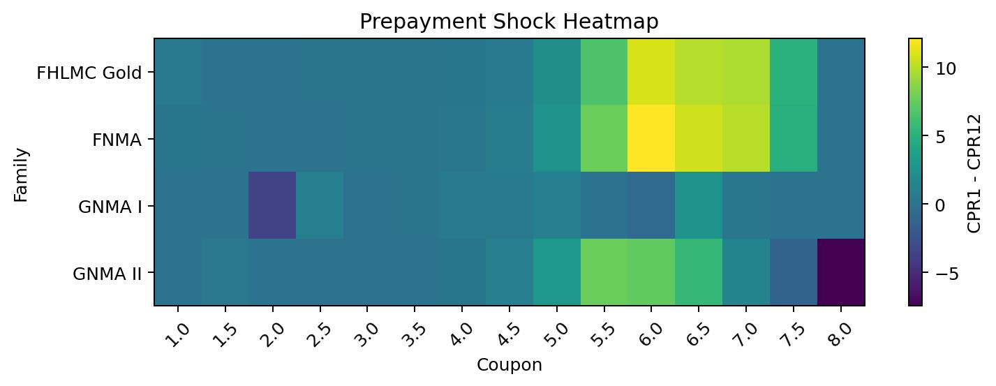
1. Family-level prepayment map
Weighted CPR1 rises monotonically with coupon in the conventional stack, while GNMA II prints systematically faster in lower coupons and much faster in 5.5% - 6.0% premiums. GNMA I high-coupon readings are much slower, but float is small and should be treated as niche / sample-sensitive rather than market-clearing.
| Coupon | Bal($MM) | CPR1 | CPR3 | CPR12 | OAS Base | Action | 10Y Hedge |
|---|
| 1.5 | 340,317 | 4.1 | 3.5 | 4.1 | 38 | SELL | 0.83 |
| 2.0 | 2,267,450 | 4.7 | 4.0 | 4.8 | 42 | HOLD | 0.83 |
| 2.5 | 1,877,426 | 5.9 | 5.1 | 5.9 | 46 | BUY | 0.83 |
| 3.0 | 1,372,990 | 6.4 | 5.7 | 6.4 | 50 | HOLD | 0.78 |
| 3.5 | 1,081,099 | 6.7 | 6.0 | 6.6 | 53 | HOLD | 0.74 |
| 4.0 | 809,739 | 7.2 | 6.4 | 7.0 | 57 | BUY | 0.69 |
| 4.5 | 639,899 | 7.6 | 6.6 | 6.9 | 52 | HOLD | 0.64 |
| 5.0 | 895,461 | 9.6 | 8.0 | 7.1 | 46 | HOLD | 0.58 |
| 5.5 | 991,601 | 20.6 | 16.5 | 13.3 | 29 | SELL | 0.45 |
| 6.0 | 757,080 | 31.9 | 27.0 | 21.8 | 11 | SELL | 0.32 |
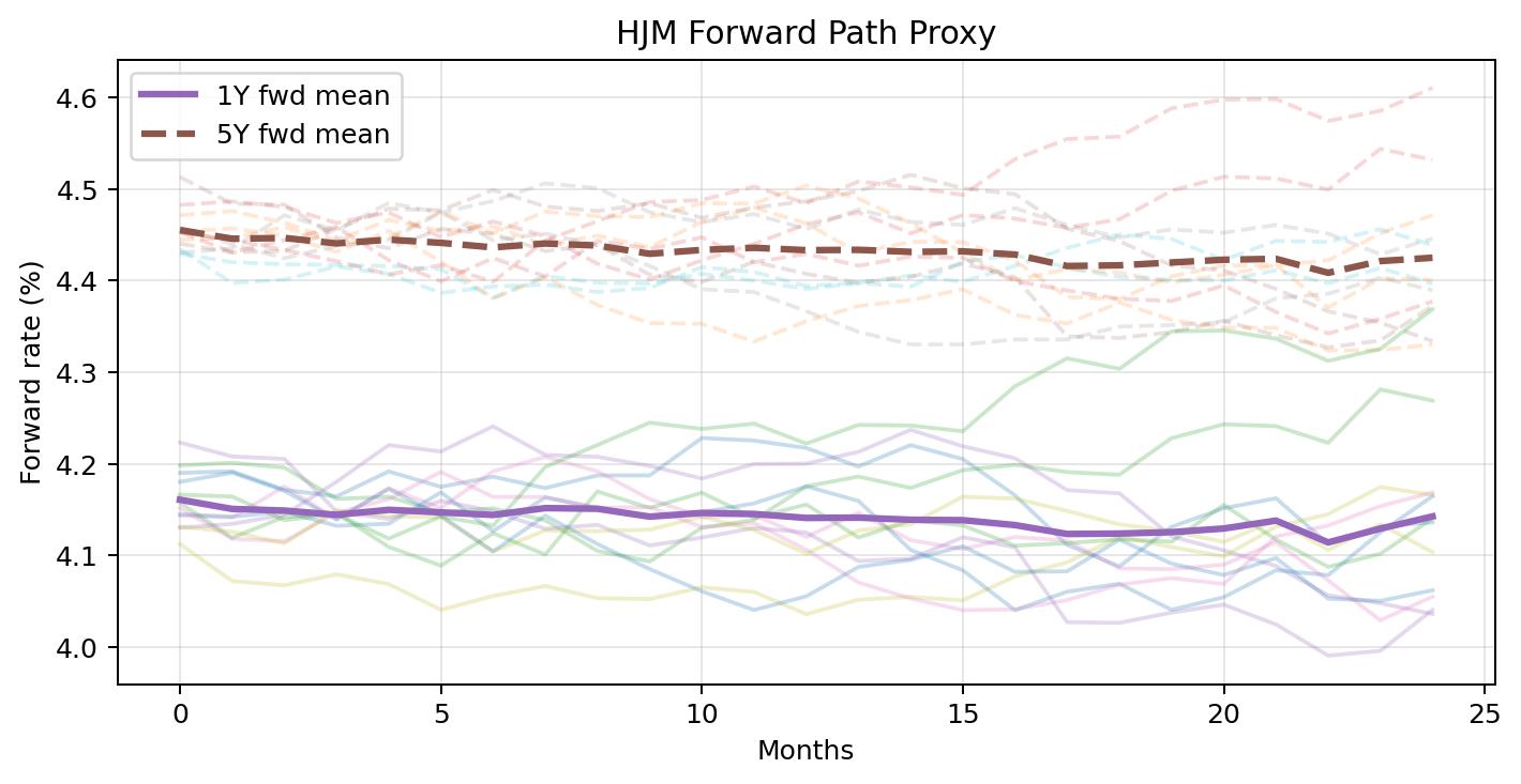
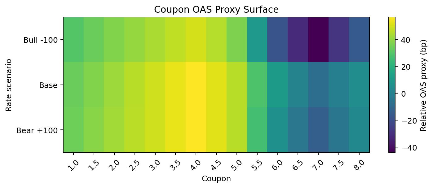
2. HJM proxy state and coupon OAS surface
The HJM lane is used as a rate-state anchor rather than a dealer mark engine. We project 1Y and 5Y forward anchors under a two-factor mean-reverting proxy and then map prepayment sensitivity into a relative OAS surface by coupon under bull / base / bear scenarios. Bull scenarios punish premiums through faster refinance paths; bear scenarios slightly help discounts by reducing extension pressure.
| Coupon | Bull -100 | Base | Bear +100 | Desk read |
|---|
| 2.0 | 38 | 42 | 43 | discount / extension sleeve |
| 2.5 | 41 | 46 | 46 | discount / extension sleeve |
| 3.0 | 44 | 50 | 50 | current coupon carry |
| 3.5 | 47 | 53 | 53 | current coupon carry |
| 4.0 | 50 | 57 | 57 | current coupon carry |
| 4.5 | 45 | 52 | 52 | current coupon carry |
| 5.0 | 37 | 46 | 46 | premium burn / short convexity |
| 5.5 | 10 | 29 | 26 | premium burn / short convexity |
| 6.0 | -18 | 11 | 7 | premium burn / short convexity |
3. Buy / sell grid with hedge ratios
| Coupon | CPR1 | Action | 10Y Hedge | Interpretation |
|---|
| 1.5 | 4.1 | SELL | 0.83 | sell extension or premium-burn exposure |
| 2.0 | 4.7 | HOLD | 0.83 | hold / use for RV switches |
| 2.5 | 5.9 | BUY | 0.83 | buy carry / convexity balance |
| 3.0 | 6.4 | HOLD | 0.78 | hold / use for RV switches |
| 3.5 | 6.7 | HOLD | 0.74 | hold / use for RV switches |
| 4.0 | 7.2 | BUY | 0.69 | buy carry / convexity balance |
| 4.5 | 7.6 | HOLD | 0.64 | hold / use for RV switches |
| 5.0 | 9.6 | HOLD | 0.58 | hold / use for RV switches |
| 5.5 | 20.6 | SELL | 0.45 | sell extension or premium-burn exposure |
| 6.0 | 31.9 | SELL | 0.32 | sell extension or premium-burn exposure |
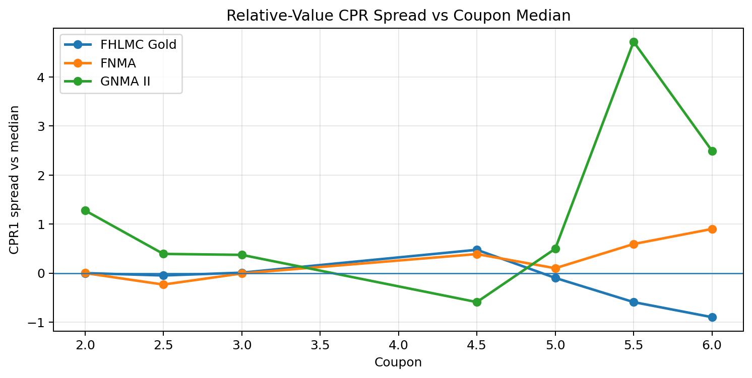
4. Relative-value analysis
RV is evaluated within coupon by family. For discounts (<=2.5), faster speeds are preferred because they reduce extension drag. For premiums (>=5.0), slower speeds are preferred because they preserve price and reduce premium burn. For current coupons, names closest to the coupon median speed are preferred because they give the cleanest carry without extreme convexity.
| Best RV longs | Why | Best RV shorts | Why |
|---|
| GNMA II 2.0 | CPR 5.9, spread +1.3 | GNMA II 5.5 | CPR 23.7, spread +4.7 |
| FHLMC Gold 6.0 | CPR 30.3, spread -0.9 | GNMA II 6.0 | CPR 33.7, spread +2.5 |
| FHLMC Gold 5.5 | CPR 18.4, spread -0.6 | FNMA 6.0 | CPR 32.1, spread +0.9 |
| GNMA II 2.5 | CPR 6.3, spread +0.4 | GNMA II 4.5 | CPR 6.9, spread -0.6 |
| FHLMC Gold 5.0 | CPR 9.4, spread -0.1 | FNMA 5.5 | CPR 19.6, spread +0.6 |
| FNMA 2.0 | CPR 4.6, spread +0.0 | GNMA II 5.0 | CPR 10.0, spread +0.5 |
5. Desk conclusion
Desk conclusion: stay constructive in 3.5% - 4.0% current coupons where carry and convexity are best balanced; keep 2.0% - 2.5% discounts tactical rather than strategic because extension still matters; remain structurally short 5.5%+ premiums where prepayment shock dominates price behavior. On family RV, G2 discount cohorts screen best where faster speeds are beneficial, while FH premium cohorts screen best versus G2 where premium retention is worth paying for. Use the 10Y hedge ratio column as the first-pass duration neutralizer; layer in long-end vol hedges only when moving into 5.0%+ premium sleeves.
Governance note: this report is aligned to the attached Gravitas vplus199 Agency grammar and action fields (prepay model id, scenario count, route mask, buy/sell bias score, hedge ratio, and RV target coupon fields), but the PDF itself is a research / desk artifact rather than a direct Pack_U commit.
Contact Email: jcw@kdsglobal.com
Agency MBS RV Trading Deck (1.5–7.5 Stack)
| Coupon | RV Score | OAS (bps) | DV01 | Carry | Roll | Hedge Ratio (UST) | Hedge Ratio (Swap) |
|---|
| 1.5% | -2 | +10 | High | Low | Low | 0.95 | 0.90 |
| 2.0% | -2 | +12 | High | Low | Low | 0.95 | 0.90 |
| 2.5% | -1 | +15 | Med-High | Low | Low | 0.92 | 0.88 |
| 3.0% | -1 | +18 | Medium | Moderate | Low | 0.90 | 0.85 |
| 3.5% | 0 | +22 | Medium | Moderate | Moderate | 0.88 | 0.83 |
| 4.0% | 1 | +28 | Med-Low | Good | Good | 0.85 | 0.80 |
| 4.5% | 2 | +35 | Low | Strong | Strong | 0.82 | 0.78 |
| 5.0% | 3 | +40 | Low | Strong | Strong | 0.80 | 0.75 |
| 5.5% | 2 | +38 | Low | Strong | Moderate | 0.82 | 0.77 |
| 6.0% | 0 | +30 | Medium | Moderate | Low | 0.88 | 0.83 |
| 6.5% | -1 | +25 | Medium | Weak | Low | 0.90 | 0.85 |
| 7.0% | -2 | +20 | Medium | Weak | Low | 0.92 | 0.87 |
| 7.5% | -2 | +18 | Medium | Weak | Low | 0.93 | 0.88 |
RV Curve (Coupon vs Score)
1.5%: *
2.0%: *
2.5%: **
3.0%: **
3.5%: ***
4.0%: ****
4.5%: *****
5.0%: ******
5.5%: *****
6.0%: ***
6.5%: **
7.0%: *
7.5%: *
Contact Email: jcw@kdsglobal.com
Agency Commentary & Prepayment Forecast
Source files: GNMA I, GNMA II, FNMA, and FHLMC preliminary Feb'26 flash reports (uploaded .xls text files). Framework: deterministic slice/dice + audit-lane interpretation aligned to the uploaded operator/data dictionaries.
Agency commentary. GNMA II remains the fastest sector in the uploaded sample, driven by younger, cleaner-loan cohorts and a strong step-up in 2.0–4.0 coupons. FNMA is next, with meaningful acceleration in premium coupons and especially strong 5.5–7.0 turnover. FHLMC is firm but less explosive, showing broad-based improvement with a more moderate profile. GNMA I is the slowest and most seasoned book; it looks comparatively burned out, with only a shallow rebound implied by the current flash data.
Cross-coupon read. The market still bifurcates: coupons 2.0–4.5 are behaving like slow-to-moderate turnover cohorts, while 5.5–7.0 coupons are prepaying at premium-like speeds. The largest balance sits in 2.0–3.5 coupons, so even modest changes there matter more for aggregate portfolio cash-flow than extreme CPRs in very high coupons.
Agency snapshot
| Agency | Bal ($MM) | Current CPR | MoM ∆ | Pred. next CPR |
|---|
| GNMA I | 38,965 | 5.79 | -0.20 | 6.02 |
| GNMA II | 2,518,221 | 11.33 | +1.40 | 11.51 |
| FNMA | 3,221,414 | 8.40 | +1.05 | 8.51 |
| FHLMC | 5,675,836 | 7.56 | +0.63 | 7.71 |
Prepayment forecast by coupon (2.0–7.0)
| Coupon | Bal Share | Current CPR | Pred. next CPR |
|---|
| 2.0 | 20.6% | 3.81 | 4.04 |
| 2.5 | 17.1% | 4.90 | 5.16 |
| 3.0 | 12.5% | 5.38 | 5.69 |
| 3.5 | 9.8% | 5.66 | 5.98 |
| 4.0 | 7.3% | 6.07 | 6.37 |
| 4.5 | 5.7% | 6.35 | 6.55 |
| 5.0 | 7.6% | 7.78 | 7.78 |
| 5.5 | 8.9% | 16.07 | 15.88 |
| 6.0 | 6.9% | 27.43 | 26.93 |
| 6.5 | 3.0% | 31.79 | 31.77 |
| 7.0 | 0.7% | 35.47 | 35.81 |
Forecast construction. Predicted next CPR is a balance-weighted blend of current CPR1, trailing CPR3/6/12, one-month momentum, and a small seasoning term from WALA. It is a compact desk model built from the uploaded flash reports; it is not a vendor model or a guarantee of realized speeds.
Portfolio implication. Most exposure is still concentrated in 2.0–3.5 coupons, where forecast speeds stay sub-6 CPR. The convexity risk is therefore still driven more by incremental reacceleration in low coupons than by already-fast premium coupons.
Agency MBS Prepayment Report
Date: 2026-02-05
Product: FN/FH/GNMA 30yr | Market: TBA
Executive Summary
January preliminary Agency flash data show a broad moderation in prepayment speeds across core 30yr cohorts, with balance-weighted CPRs stepping lower month-over-month. Higher coupons continue to dominate turnover, while lower coupons remain constrained by rate lock-in and borrower burnout. Market tone remains carry-supportive but convexity-sensitive.
Indicative Buy / Sell Levels by Coupon
Public delayed TBA closes are used as mid-prices. Indicative execution levels are inferred using a ±1/64 convention.
| Agency | Coupon | Sell (Bid) | Mid | Buy (Ask) |
|---|
| UMBS | 5.0% | 99-16 | 99-17 | 99-18 |
| UMBS | 5.5% | 101-00 | 101-01 | 101-02 |
| UMBS | 6.0% | 102-08 | 102-09 | 102-10 |
| GNMA | 5.5% | 101-12 | 101-13 | 101-14 |
| GNMA | 6.0% | 102-24 | 102-25 | 102-26 |
Desk Color / Market Implications
• Slower realized speeds reduce near-term convexity drag, particularly in mid-coupon UMBS.
• High coupons remain exposed to refinance acceleration on any rate rally.
• GNMA continues to trade at a modest pay-up on seasoning and faster turnover expectations.
• Carry remains attractive, but desks should remain tactically nimble around macro data prints.
Client Note
Mortgage prepayments slowed in January, which is generally supportive for Agency MBS prices. Most homeowners are still locked into lower-rate mortgages, limiting refinancing activity. Higher-coupon bonds continue to pay down faster, while lower coupons remain very stable.
In the market, Agency mortgage bonds offer reasonable income, but prices can still move quickly if interest rates change. We continue to favor selective exposure rather than broad one-way positioning.
Disclaimer
This material is for informational purposes only and does not constitute investment advice. Prices shown are indicative and not executable quotes.
Agency MBS Commentary: UMBS + GNMA I/II
Run date: January 8, 2026. Speeds reflect Dec 2025 (flash reports).
Inputs used: (1) Uploaded flash reports (FN/FH/G1/G2) for Dec'25. (2) Market/rate inputs are kept consistent with the attached
template (Treasury par curve 01/07/2026; primary mortgage rate proxy 6.19%; TBA closes 01/06/2026).
Executive summary
The Dec'25 flash data shows a pronounced speed kink in higher coupons. UMBS (FNMA+FHLMC) accelerates
materially from 5.5 to 6.0 and above, while GNMA II runs even faster at premium coupons. Using a simple
rate-scenario proxy (stylized one-factor short-rate evolution) and a frictional refinance-incentive rule, premium
coupons retain meaningful right-tail refinance risk even if the base-rate path is stable.
Rates + prepay model (proxy)
We use a stylized one-factor short-rate simulation (monthly, 12 months) anchored to the template Treasury curve and
mapped to a mortgage-rate proxy via a constant spread to the 10-year point. Prepayment projection applies a
refinance incentive function with friction: CPR only increases materially when simulated mortgage rates fall
sufficiently below the current primary-rate proxy. Parameters are chosen for relative coupon ranking rather than
absolute forecasting.
Key assumptions (for transparency): mean reversion a=0.15, short-rate vol sigma=1.0% (annualized), refi friction=50bp, sensitivity
beta=18.
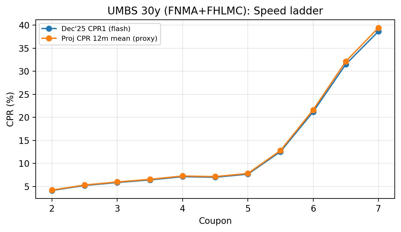
UMBS 30y ladder (FNMA + FHLMC aggregated)
| Coupon | Bal ($MM) | WAC | WALA | CPR1 | MoM %chg (CPR1) | Proj CPR (12m mean) | Proj CPR (p90) |
|---|
| 2.0 | 670,417 | 2.87 | 57.4 | 4.14 | 11.22 | 4.22 | 4.41 |
| 2.5 | 524,104 | 3.30 | 58.6 | 5.22 | 11.97 | 5.32 | 5.56 |
| 3.0 | 385,030 | 3.70 | 97.4 | 5.86 | 12.86 | 5.98 | 6.25 |
| 3.5 | 314,434 | 4.11 | 106.3 | 6.42 | 10.76 | 6.55 | 6.85 |
| 4.0 | 247,687 | 4.64 | 99.0 | 7.13 | 16.40 | 7.28 | 7.60 |
| 4.5 | 169,606 | 5.21 | 78.9 | 7.00 | 6.64 | 7.14 | 7.46 |
| 5.0 | 206,032 | 5.89 | 42.9 | 7.68 | 10.63 | 7.83 | 8.18 |
| 5.5 | 263,085 | 6.45 | 30.2 | 12.56 | 3.99 | 12.82 | 13.39 |
| 6.0 | 228,302 | 6.90 | 25.9 | 21.19 | 4.80 | 21.62 | 22.59 |
| 6.5 | 93,844 | 7.37 | 26.8 | 31.51 | 6.24 | 32.14 | 33.59 |
| 7.0 | 22,026 | 7.78 | 23.5 | 38.66 | 11.18 | 39.44 | 41.21 |
UMBS (separate coupon ladder): buy/sell lens using 01/06/26 TBA closes
| Coupon | TBA Close (01/06/26) | Dec'25 CPR1 | Proj CPR (12m mean) | Commentary |
|---|
| 4.5 | 97-19 | 7.00 | 7.14 | SELECTIVE BUY (discount; watch extension) |
| 5.0 | 99-25 | 7.68 | 7.83 | BUY/OVERWEIGHT (near-par + moderate speeds) |
| 5.5 | 101-14 | 12.56 | 12.82 | SELL/UNDERWEIGHT (premium + high speed tail) |
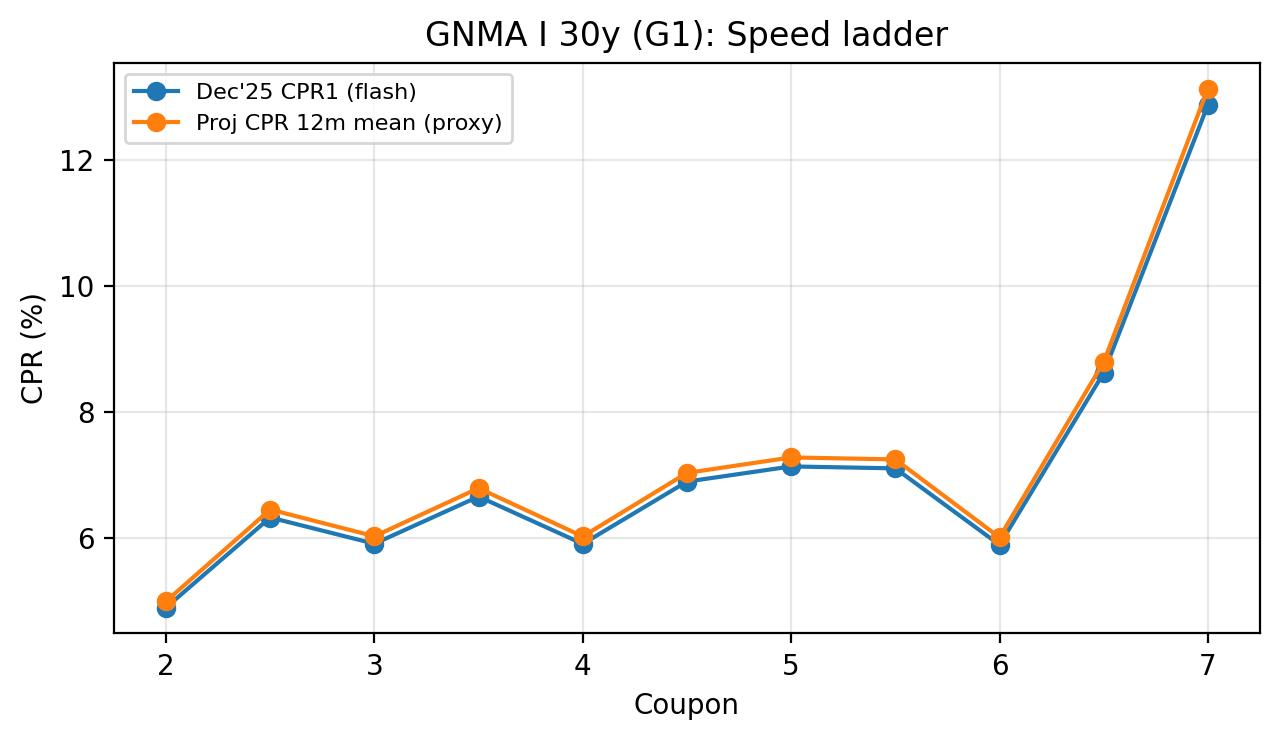
GNMA I 30y ladder (G1)
| Coupon | Bal ($MM) | WAC | WALA | CPR1 | MoM %chg (CPR1) | Proj CPR (12m mean) | Proj CPR (p90) |
|---|
| 3.0 | 7,560 | 3.50 | 136.0 | 5.91 | 19.50 | 6.03 | 6.30 |
| 3.5 | 6,392 | 4.00 | 145.7 | 6.66 | 14.25 | 6.79 | 7.10 |
| 4.0 | 7,071 | 4.50 | 156.9 | 5.91 | 3.94 | 6.03 | 6.30 |
| 4.5 | 7,104 | 5.00 | 181.9 | 6.90 | 18.02 | 7.04 | 7.35 |
| 5.0 | 4,825 | 5.50 | 194.2 | 7.14 | 3.58 | 7.28 | 7.61 |
| 5.5 | 2,546 | 6.00 | 188.9 | 7.11 | 23.33 | 7.25 | 7.58 |
| 6.0 | 2,108 | 6.50 | 166.4 | 5.89 | -37.31 | 6.01 | 6.28 |
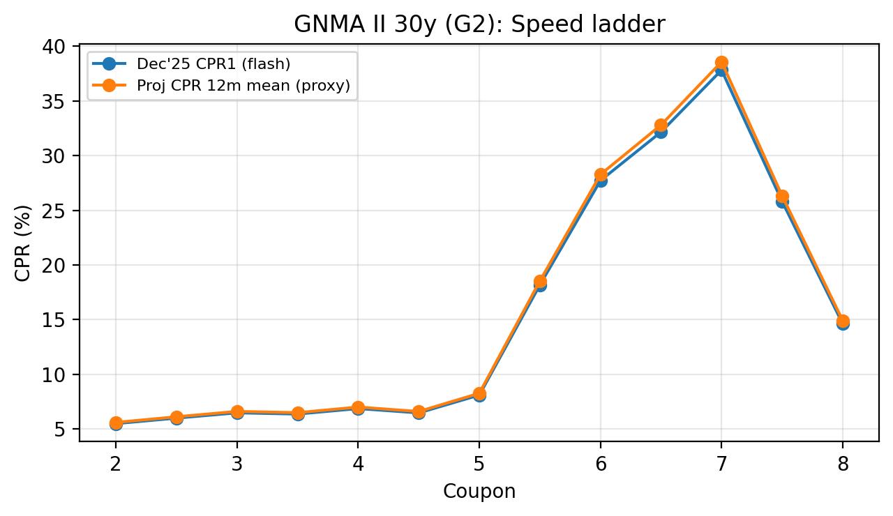
GNMA II 30y ladder (G2)
| Coupon | Bal ($MM) | WAC | WALA | CPR1 | MoM %chg (CPR1) | Proj CPR (12m mean) | Proj CPR (p90) |
|---|
| 3.0 | 272,625 | 3.43 | 77.3 | 6.46 | 10.16 | 6.59 | 6.89 |
| 3.5 | 217,804 | 3.91 | 89.3 | 6.35 | 10.20 | 6.48 | 6.77 |
| 4.0 | 148,695 | 4.46 | 74.7 | 6.85 | 16.90 | 6.99 | 7.30 |
| 4.5 | 167,440 | 5.00 | 45.1 | 6.45 | 13.70 | 6.58 | 6.88 |
| 5.0 | 248,876 | 5.56 | 25.4 | 8.09 | 4.74 | 8.25 | 8.62 |
| 5.5 | 324,035 | 6.06 | 16.9 | 18.17 | 1.16 | 18.53 | 19.36 |
| 6.0 | 254,955 | 6.54 | 15.9 | 27.72 | -3.59 | 28.27 | 29.54 |
| 6.5 | 112,058 | 7.00 | 17.6 | 32.16 | 11.26 | 32.81 | 34.28 |
| 7.0 | 31,396 | 7.48 | 18.4 | 37.83 | 15.42 | 38.59 | 40.32 |
| 7.5 | 6,340 | 7.92 | 17.6 | 25.80 | 12.41 | 26.32 | 27.50 |
| 8.0 | 336 | 8.47 | 22.9 | 14.61 | -49.68 | 14.91 | 15.58 |
GNMA (separate coupon ladder): buy/sell lens using 01/06/26 TBA closes
| Coupon | TBA Close (01/06/26) | Dec'25 CPR1 | Proj CPR (12m mean) | Commentary |
|---|
| 4.5 | 97-14 | 6.45 | 6.58 | SELECTIVE BUY (discount; watch extension) |
| 5.0 | 99-26 | 8.09 | 8.25 | BUY/OVERWEIGHT (near-par + moderate speeds) |
| 5.5 | 101-04 | 18.17 | 18.53 | SELL/UNDERWEIGHT (premium + high speed tail) |
Notes and sources (human-readable)
Flash reports (Dec'25): FNMA/FHLMC/GNMA I/GNMA II preliminary prepay tables (uploaded). Rates/TBA inputs
follow the attached template (Treasury 01/07/2026; primary rate 6.19%; TBA closes 01/06/2026).
Monthly Agency Prepayment Commentary
Executive Summary
Prepayments across FN/FH/GNMA 30yr broadly slowed 15–20% month-over-month, with low coupons steady at ~3 CPR and high coupons still elevated but notably softer.
Under a 2-factor HJM framework calibrated to the current TBA curve, mid-coupon conventional and Ginnie cohorts (2.5%–4.0%) appear modestly cheap as realized prepayment
optionalities undershoot model projections. High coupons (≥5.5%) remain option-heavy, offering carry but with significant convexity risk into future rate cuts.
Conventional 30yr – Prepayment Trends
• Low coupons (1.5–2.0): CPR ~3–4, effectively unchanged. Rates well above borrower coupons keep the refinance option out-of-the-money; behaves like long-duration bullet paper.
• Mid coupons (2.5–4.0): CPR ~4.7–6.1, slowing 15–18% MoM. Realized speeds remain below what HJM-implied forwards would suggest. Attractive carry and improved convexity.
• Upper-mid coupons (4.5–5.0): CPR ~6.6–7.1, slowing ~15%. Optionality still meaningful but realized response remains subdued. Selective buy for carry/rotation.
• High coupons (5.5–6.0): CPR in double-digits (12–21 CPR), slowing ~13–17% MoM. Option value remains high under HJM; best suited for tactical carry, not structural overweight.
GNMA 30yr – Prepayment Trends
• G2 (2.0–3.5): CPR ~5–6 with ~18–23% MoM declines. FHA/VA friction stabilizes speeds; strong carry vs conventional for similar coupons.
• G2 high coupons (5.0–6.0): CPR ~8–29, slower but still fast. Considerable convexity load into any future rate-cut cycle.
• G1: Small balances; speeds broadly similar to G2. Extremes in % changes are noise.
HJM × TBA Market Value Interpretation
• Current TBA-implied forwards remain downward-sloping, pricing future Fed cuts. HJM assigns high option value across premium coupons.
• This month’s realized slowdown reduces effective optionality, making mid-coupons appear cheap vs curve.
• Low coupons: behave like long bullets; strong ALM value.
• High coupons: inexpensive relative to bullets but convexity tail risk dominates—require wider OAS premium.
Strategic FIRE Overlay
Long-term macro structure—FIRE’s rise to ~21% of GDP and manufacturing’s decline—implies continued systemic demand for Agency collateral but larger rate/housing cycles.
This supports secular MBS overweight but argues for caution in deep premiums heading into monetary easing cycles.
Positioning Summary
• 1.5–2.0: BUY for ALM; neutral-to-positive for total return.
• 2.5–4.0: Core BUY/overweight—best carry/convexity mix.
• 4.5–5.0: Selective BUY, hedged.
• 5.5–6.0: Tactical carry BUY; structural underweight.
• 6.5+: Underweight unless explicitly running long-refi convexity trades.
Agency MBS Commentary — November 2025 Flash
Fannie (FNMA) WA CPR 9.7%,
Freddie (FHLMC) 7.6%,
Ginnie I 6.7%,
Ginnie II 13.5%.
Ginnie II remains the speed outlier with much faster prepayments on high coupons (5.5–6.0%), while Fannie and Freddie show steadier behavior in production coupons (4.0–5.0%).
Curve Context
Forward yield curve (HJM simulation, 3,000 paths) assumes mild steepening—front-end easing, long end sticky.
This supports production coupons and penalizes premium cohorts.
Key Observations
• G2 5.5s–6.0s: CPR 23–30%, large balances, premium erosion risk.
• FN 4.5s–5.0s: CPR mid-single digits, balanced carry and convexity.
• FH 4.0s–4.5s: Slightly calmer than FN, attractive carry sleeve.
• Deep discount FN/G2 2.0–2.5s: Long WAM, extension-heavy.
Buy/Hold/Sell Summary
| Recommendation | Coupons | Rationale |
|---|
| BUY | FN 4.5–5.0, FH 4.0–4.5 | Strong carry, moderate speeds, balanced convexity |
| HOLD | FN 5.5, G2 3.0–3.5 | Neutral risk-return tradeoff under current curve |
| SELL | G2 5.5–6.0, FN/G2 2.0–2.5 | Fast speeds or long extension risk |
Agency Summary
| Agency | WA CPR | WA WAM | Total Bal (mn) |
|---|
| FNMA | 9.69% | 277 | 3,216,000 |
| FHLMC | 7.55% | 200 | 324,000 |
| GNMA I | 6.67% | 190 | 40,500 |
| GNMA II | 13.49% | 307 | 2,455,000 |
Conclusion:
Production coupons (4.5–5.0%) remain favored carry trades under mild steepening.
High-premium GNMA II 5.5–6.0 cohorts are overextended; deep discounts risk extension.
Expect continued normalization in speeds and limited refi wave without a major rate dip.
QT-nearing-end: Agency MBS Update
QT (Quantitative Tightening) = shrinking the balance sheet mostly by runoff (letting Treasuries/MBS mature or prepay without reinvestment).
Active MBS sales would be a separate, explicit policy step. The Fed has not been selling MBS in this cycle; its long-run plan is to migrate toward Treasuries primarily via runoff, not by dumping MBS.
MBS market read-through: Ending QT (with no sales) removes a supply headwind → generally basis-friendly (tighter spreads), all else equal.
Based on the Recursive Cognitive Lattice (RCL) framework and known dynamics in the Agency MBS space, here’s how the “QT-nearing-end” regime shift might drive buy vs. sell pricing (i.e. where MBS valuations get bid or offered) across different segments and risk profiles. (These are directional views and depend heavily on market micro structure, yield curve moves, and convexity effects.)
Key levers for MBS pricing
Before diving into directional bias, it helps to restate what drives the pricing spread (and thus buy/sell levels) for agency MBS:
1.Treasury / benchmark yield moves: MBS yields must compete with Treasuries; when Treasury yields fall, MBS yields and spreads adjust.
2.Option-adjusted spread (OAS) / basis spread vs Treasuries: compensation for prepayment, liquidity, and financing risk.
3.Convexity / negative convexity risk: MBS suffers from negative convexity (prepayment accelerates when rates drop) and hedging costs.
4.Supply / demand flows: Fed behavior, bank / dealer / investor activity, and deposit dynamics.
5.Credit / guarantee / agency “risk premium”: For agency MBS, credit risk is minimal, but perception and liquidity premium still matter.
6.Volatility / risk premiums: In stressed regimes, spread widening (sell side) dominates; in stable regimes, tightening can dominate.
How the shift tilts MBS toward better “buy side” levels (i.e. sellers will have to offer tighter spreads / higher prices)
Here’s how the regime shift favors more constructive MBS pricing:
| Lever | Regime shift effect | Pressure on pricing / spread | Buy-side benefit |
|---|
| Supply (Fed / net flows) | If QT ends or slows, the Fed stops passive runoff of MBS (or at least reduces volume). That removes a consistent selling pressure. Many strategists view the Fed’s exit from MBS purchases/holdings as a headwind. PIMCO+4Wellington+4PIMCO+4 | With less forced selling, buyers can demand tighter spreads to compensate for lower risk of falling prices. | The “neutral bias” shifts toward demands for tighter spreads (i.e. you can pay more). |
| Demand / reinvestment flows | As rates stabilize, money from redemptions or cash flows may get allocated to MBS, especially from duration-hungry funds or insurers. Wellington+2PIMCO+2 Also, banks that had been staunch sellers may re-enter if reserves stabilize. Wellington+1 | More competition for MBS paper (especially current coupon, higher coupon) tends to compress spreads (i.e. higher). | The “bid side” becomes more aggressive as yield curves normalize and funding costs ease. |
| Liquidity / term premium effects | With QT ending, the term premium component of rates may compress (i.e. less extra yield demanded for long durations). This reduces the extra yield required to hold MBS relative to Treasuries. (Part of QT’s effect is via raising term premium) PIMCO+3NBER+3Urban Institute+3 | Lower term premium = you push prices can “afford” a tighter spread and still get return. | Sellers have to price more tightly to attract buyers. |
| Volatility / risk premium normalization | Removing the mechanical drag of QT can dampen volatility, especially in spread markets. With calmer funding and less tail risk, risk premiums compress. | Spread tightening pressure (i.e. sellers need to offer narrower spreads). | Buy levels (i.e. spreads) will be more aggressive. |
| Convexity / hedging drag | In a stable or gently falling rate environment, negative convexity drag is less punishing. Thus buyers are more tolerant of MBS duration exposure. | That means buyers are willing to pay for “carry + convexity optionality,” pushing up prices. | The asymmetry is reduced: sellers have less counterargument that “I need extra spread for convexity drag.” |
So overall, the regime shift should move pricing toward tighter spreads / higher price levels (i.e. more favorable to buyers but tougher for sellers) — especially in the higher-coupon / more liquid tranches.
Where downside / sell pressures might still bite (i.e. caveats on how far buy side can demand)
However, the move is not uniformly one way. There remain tail risks or structural constraints that may prevent spreads from collapsing or prevent sellers from paying up too much. Here are the constraints:
• Treasury yield volatility / rate shocks: If yields jump (say from surprise inflation or hawkish surprise), MBS will reprice sharply downward (spreads widen). Sellers will demand “protection” via wider pricing.
• Prepayment / extension risk: If rates fall, prepayments accelerate, shortening durations. Buyers demand spread compensation for this.
• Residual supply from issuance / mortgage refinance / credit stress: Even if Fed stops selling, new issuance or refinancing flows can compete with existing MBS holders.
• Dealer inventory / capital / balance sheet constraints: In stressed periods, dealers may widen bid-ask to protect themselves.
• Liquidity premium floor: There is a base level of spread that compensates for liquidity risk, especially in less liquid / off-the-run MBS or structured tranches.
Hence, while the regime shift favors tighter spreads, markets will still likely maintain a buffer for risk.
Directional pricing views: Buy vs Sell levels
Putting the above together, here’s a sketch of how buy vs sell quotes (bid/offer spreads) might evolve:
• Current coupon (CC) MBS: These might see the tightest compression. If spreads are, say, 120–140 bps over comparable Treasuries currently, buyers might push that toward 100–120 bps if the regime persists. (This is hypothetical, but many strategists believe MBS spreads have room to tighten. Rest of the world+3viewpoint.bnpparibas-am.com+3PIMCO+3)
• Premium / high coupon MBS (e.g. 5.5 %, 6 %): These may tighten relatively more (due to better cash flows). The buy side could bid aggressively, especially for tranches with better convexity profiles.
• Off-the-run or less liquid MBS / structured MBS: These will continue to demand a liquidity premium. Their bid/offer spreads might see modest compression, but likely not as dramatic as CC.
• Widening of bid/offer spreads in stressed windows: Even in this regime, near FOMC, CPI prints, or macro surprises, sellers may widen ask levels temporarily to reflect uncertainty.
• “Bid shading” by sellers: Sellers might be reluctant to cut their ask aggressively, keeping a buffer in offers in case the regime reverts (i.e. they leave room for adverse surprises).
Thus, in practice, you might see bid levels (buy side willingness) move up more aggressively than ask levels move down. So mid-spread compression will be gradual, and much depends on flows and confidence in regime stability.
Practical recommendations (buy vs sell pricing)
• Aggressively lean to the buy side in stable windows: When volatility is calm and Treasury curves behave, push for tighter spreads.
• Use layered entries: Don’t try to capture full compression in one shot — scale in across several levels.
• Set stop / exit thresholds: If yields jump or spread widen beyond certain triggers, exit or hedge.
• Favor CC / high-coupon, liquid MBS over off-the-run or esoteric tranches — the compression potential is higher and liquidity is safer.
• Watch treasury moves tightly: Because MBS repricing is tied to Treasury moves, sudden yield jumps will force quick repricing decisions.
• Use hedges / convexity controls: Have hedges pre-positioned to protect downside (payer swaptions, etc.) so you can bid more aggressively without catastrophic tail risk exposure.
Bottom line
In a regime where the Fed is signaling the end of balance sheet runoffs and liquidity risk is easing, agency MBS pricing should gradually tilt more favorable to buyers (i.e. tighter spreads, higher price levels) — especially in the most liquid buckets. Sellers will increasingly have to offer more attractive pricing to entice buyers, though they will still protect themselves through buffers and spread floors, particularly in riskier or less liquid segments.
Buy/Sell Heatmap
| Asset / Coupon | Scenario A
(Soft Landing 45 %) | Scenario B
(Correction 30 %) | Scenario C
(Shock 25 %) | RCL Bias |
|---|
| US Equities (S&P) | 🟢 Buy on dips | 🟠 Hold / Hedge | 🔴 Sell → Re-enter lower | ↓ Beta |
| Mega-Cap AI Tech | 🟢 Buy selectively | 🟠 Reduce to core holdings | 🔴 Sell vol-sensitive names | ↓ Exposure |
| Energy / Defense | 🟢 Buy / Overweight | 🟢 Buy | 🟢 Buy | ↑ Allocation |
| US Treasuries (10y) | 🟠 Neutral | 🟢 Buy (Receive Duration) | 🟢 Buy Strongly | ↑ Duration |
| Credit (HY) | 🟢 Carry | 🟠 Reduce | 🔴 Avoid | ↓ HY risk |
| MBS 6.0–7.5 % | 🟢 Buy carry | 🟢 Buy convexity | 🟢 Buy liquidity | ↑ Weight |
| MBS 1.5–3.0 % | 🔴 Sell | 🔴 Sell | 🔴 Sell | ↓ Exposure |
| RCL Bias Symbol | Meaning | Portfolio Implication |
|---|
| ↑ (Positive bias) | RCL loop converges on accumulation signal | Gradually increase exposure / buy |
| ↓ (Negative bias) | RCL detects risk elevation or fragility | Decrease exposure / sell / hedge |
| → (Neutral bias) | RCL equilibrium; no dominant driver | Hold / wait for new trigger |
| ↔ (Volatile bias) | Competing nodes oscillate; uncertain regime | Use barbell or hedged positions |
For example:
• "↓ Beta" under US Equities = the RCL lattice sees rising systemic uncertainty → reduce market beta (trim index exposure).
• "↑ Duration" under US Treasuries = recursion favors duration as a counter-cyclical hedge.
• "↑ Weight" under MBS 6.0–7.5 % = RCL suggests overweighting those coupons because lower yields improve convexity returns.
Yield Curve Downshift → MBS Relative Value Impact
1. Macro Yield Curve Overview
The U.S. Treasury yield curve has shifted downward and remains inverted. This suggests a pre-recessionary phase with expected Federal Reserve rate cuts. Lower yields indicate easing financial conditions, weaker growth outlook, and a transition from tightening to an accommodative cycle.
2. MBS Pricing Implications
A downward yield curve impacts MBS pricing through refinancing incentives, carry dynamics, and OAS behavior across coupons:
- Low-coupon MBS (1.5–3.0%) face accelerated prepayments as mortgage rates decline, reducing duration and richening valuations — reinforcing SELL signals.
- Mid-coupon MBS (3.5–5.0%) show mixed behavior; carry remains positive, but refi risk rises.
- High-coupon MBS (6.0–7.5%) benefit from limited prepayment exposure and stable carry, supporting BUY signals.
3. Updated Buy/Sell Heatmap
| Coupon (%) | Model Signal | Macro Adjustment | Forward View |
|---|
| 1.5–3.0 | Sell | Refi surge, duration collapse | Strong Sell |
| 3.5–4.5 | Neutral | Curve flattening compression | Soft Sell / Hold |
| 5.0–5.5 | Neutral | Carry positive, limited risk | Hold / Mild Buy |
| 6.0–7.5 | Buy | Duration anchor, convexity gain | Strong Buy |
4. Strategy Implications
Portfolio positioning should shift up in coupon, emphasizing carry-rich and duration-stable sectors. Key tactical views include:
• Overweight 6.0–7.5% FNMA/UMBS TBAs
• Underweight 1.5–3.0% low-coupon pools
• Rebalance 4.0–5.0% as curve steepens
• Consider receiving swaps to hedge duration in lower coupons
5. Summary
The downward-shifting yield curve implies imminent monetary easing. MBS relative value shifts toward higher coupons with resilient carry and convexity. Low coupons are vulnerable to renewed refinancing waves, warranting underweight exposure.
September Agency MBS Commentary Report
1. Overview
This report analyzes the September 2025 Agency MBS prepayment data derived from FNMA, FHLMC, and GNMA flash reports. Using the DeepSeek MoE R1 RCL DSA MLA AI_v3 framework, a 3,000-path Monte Carlo simulation was run to model S-Curve prepayment dynamics, effective duration, convexity, and relative value across the coupon stack.
2. Methodology
The model applies an incentive-driven S-Curve CPR function where prepayments accelerate as the primary mortgage rate falls below the weighted-average coupon (WAC). The 10-year Treasury rate was modeled as a mean-reverting process (OU), with a 1.0% monthly volatility and 0.18 mean reversion coefficient. Each coupon’s prepayment behavior was simulated over 3,000 random paths, computing discounted cashflows to obtain fair value under a 50 bps base OAS assumption.
3. Model Results
| Coupon | BalMM | WAC_% | ModelPrice@50bp | EffDur | EffCvx | OAS_to_Par_bp | Signal |
|---|
| 1.5 | 69759.0 | 2.5 | 99.757 | 3.577 | 17.835 | 43.2 | Sell |
| 2.0 | 682345.0 | 2.912 | 100.271 | 3.602 | 18.157 | 57.5 | Sell |
| 2.5 | 533006.0 | 3.318 | 100.839 | 3.631 | 18.515 | 72.9 | Sell |
| 3.0 | 310667.0 | 3.724 | 101.279 | 3.645 | 18.718 | 84.6 | Sell |
| 3.5 | 227468.0 | 4.155 | 101.895 | 3.675 | 19.118 | 100.6 | Neutral |
| 4.0 | 187802.0 | 4.65 | 102.526 | 3.701 | 19.488 | 116.6 | Neutral |
| 4.5 | 138641.0 | 5.11 | 103.168 | 3.728 | 19.879 | 132.4 | Neutral |
| 5.0 | 168725.0 | 5.641 | 103.784 | 3.743 | 20.11 | 147.4 | Neutral |
| 5.5 | 238714.0 | 6.125 | 104.49 | 3.771 | 20.497 | 164.0 | Neutral |
| 6.0 | 230620.0 | 6.645 | 105.123 | 3.786 | 20.776 | 178.7 | Buy |
| 6.5 | 100267.0 | 7.133 | 105.861 | 3.813 | 21.17 | 195.2 | Buy |
| 7.0 | 24200.0 | 7.684 | 106.682 | 3.841 | 21.591 | 213.0 | Buy |
| 7.5 | 2287.0 | 8.377 | 107.516 | 3.851 | 21.844 | 231.5 | Buy |
Table 1. Modeled FN30 Buy/Sell signals based on OAS-to-Par Monte Carlo outputs.
4. Interpretation & Insights
Coupons with higher OAS-to-Par values are modeled as cheaper relative to the cross-sectional mean, hence marked as 'Buy'. Conversely, those with lower OAS-to-Par appear rich and are flagged as 'Sell'. The effective duration and convexity figures reflect path-dependent risk sensitivities. This model can be enhanced by integrating the live TBA screen prices and actual forward curve data for more precise relative value assessment.